Examples
Dynamics
Kuramoto
StDoG provides two implementations of Heun’s method. The first uses the TensorFlow. Therefore, it can be used with both CPU’s or GPU’s. The second implementation is a python wrapper to a CUDA code. The second (CUDA) is faster than TensorFlow implementation. However, a CUDA-compatible GPU is required
Creating the data and setting the variables
import numpy as np
import igraph as ig
from stdog.utils.misc import ig2sparse
num_couplings = 40
N = 20480

G = ig.Graph.Erdos_Renyi(N, 3/N)
adj = ig2sparse(G)

omegas = np.random.normal(size= N).astype("float32")
couplings = np.linspace(0.0,4.,num_couplings)
phases =  np.array([
    np.random.uniform(-np.pi,np.pi,N)
    for i_l in range(num_couplings)

],dtype=np.float32)

precision =32

dt = 0.01
num_temps = 50000
total_time = dt*num_temps
total_time_transient = total_time
transient = False
Tensorflow implementation
from stdog.dynamics.kuramoto import Heuns

heuns_0 = Heuns(adj, phases, omegas, couplings, total_time, dt,
    device="/gpu:0", # or /cpu:
    precision=precision, transient=transient)

heuns_0.run()
heuns_0.transient = True
heuns_0.total_time = total_time_transient
heuns_0.run()
order_parameter_list = heuns_0.order_parameter_list
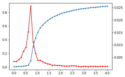
Plotting the result
import matplotlib.pyplot as plt

r = np.mean(order_parameter_list, axis=1)
stdr = np.std(order_parameter_list, axis=1)

plt.ion()
fig, ax1 = plt.subplots()
ax1.plot(couplings,r,'.-')
ax2 = ax1.twinx()
ax2.plot(couplings,stdr,'r.-')
plt.show()
CUDA implementation (faster)
For that, you need to install our another package, cukuramoto http://github.com/stdogpkg/cukuramoto
$ pip install cukuramoto
from stdog.dynamics.kuramoto.cuheuns import CUHeuns as cuHeuns

heuns_0 = cuHeuns(adj, phases, omegas,  couplings,
    total_time, dt, block_size = 1024, transient = False)

heuns_0.run()

heuns_0.transient = True
heuns_0.total_time = total_time_transient
heuns_0.run()
order_parameter_list = heuns_0.order_parameter_list
References
[1] - Thomas Peron, Bruno Messias, Angélica S. Mata, Francisco A. Rodrigues, and Yamir Moreno. On the onset of synchronization of Kuramoto oscillators in scale-free networks. arXiv:1905.02256 (2019).
Spectra
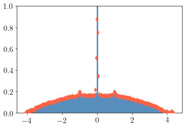
Spectral Density
The Kernel Polynomial Method can estimate the spectral density of large sparse Hermitan matrices with a computational cost almost linear. This method combines three key ingredients: the Chebyshev expansion + the stochastic trace estimator + kernel smoothing.
import igraph as ig
import numpy as np

N = 3000
G = ig.Graph.Erdos_Renyi(N, 3/N)

W = np.array(G.get_adjacency().data, dtype=np.float64)
vals = np.linalg.eigvalsh(W).real
import stdog.spectra as spectra
from stdog.utils.misc import ig2sparse

W = ig2sparse(G)
num_moments = 300
num_vecs = 200
extra_points = 10
ek, rho = spectra.dos.kpm(W, num_moments, num_vecs, extra_points, device="/gpu:0")
import matplotlib.pyplot as plt
plt.hist(vals, density=True, bins=100, alpha=.9, color="steelblue")
plt.scatter(ek, rho, c="tomato", zorder=999, alpha=0.9, marker="d")
plt.ylim(0, 1)
plt.show()
References
[1] Wang, L.W., 1994. Calculating the density of states and optical-absorption spectra of large quantum systems by the plane-wave moments method. Physical Review B, 49(15), p.10154.
[2] Hutchinson, M.F., 1990. A stochastic estimator of the trace of the influence matrix for laplacian smoothing splines. Communications in Statistics-Simulation and Computation, 19(2), pp.433-450.
Trace Functions
Given a semi-positive definite matrix \(A \in \mathbb R^{|V|\times|V|}\), which has the set of eigenvalues given by \(\{\lambda_i\}\) a trace of a matrix function is given by
The methods for calculating such traces functions have a cubic computational complexity lower bound, \(O(|V|^3)\). Therefore, it is not feasible for large networks. One way to overcome such computational complexity it is use stochastic approximations combined with a mryiad of another methods to get the results with enough accuracy and with a small computational cost. The methods available in this module uses the Sthocastic Lanczos Quadrature, a procedure proposed in the work made by Ubaru, S. et.al. [1] (you need to cite them).
Spectral Entropy
import scipy
import scipy.sparse
import igraph as ig
import numpy as np

N = 3000
G = ig.Graph.Erdos_Renyi(N, 3/N)
from stdog.spectra.trace_function import entropy as slq_entropy

def entropy(eig_vals):
s = 0.
for val in eig_vals:
    if val > 0:
    s += -val*np.log(val)
return s

L = np.array(G.laplacian(normalized=True), dtype=np.float64)
vals_laplacian = np.linalg.eigvalsh(L).real

exact_entropy =  entropy(vals_laplacian)

L_sparse = scipy.sparse.coo_matrix(L)

num_vecs = 100
num_steps = 50
approximated_entropy = slq_entropy(
    L_sparse, num_vecs, num_steps, device="/cpu:0")

approximated_entropy, exact_entropy
The above code returns
(-509.46283, -512.5283224633046)
Custom Trace Function
import tensorflow as tf

from stdog.spectra.trace_function import slq
def trace_function(eig_vals):
    return tf.exp(eig_vals)


num_vecs = 100
num_steps = 50
approximated_trace_function, _ = slq(L_sparse, num_vecs, num_steps,  trace_function)
References
1 - Ubaru, S., Chen, J., & Saad, Y. (2017). Fast Estimation of tr(f(A)) via Stochastic Lanczos Quadrature. SIAM Journal on Matrix Analysis and Applications, 38(4), 1075-1099.
2 - Hutchinson, M. F. (1990). A stochastic estimator of the trace of the influence matrix for laplacian smoothing splines. Communications in Statistics-Simulation and Computation, 19(2), 433-450.